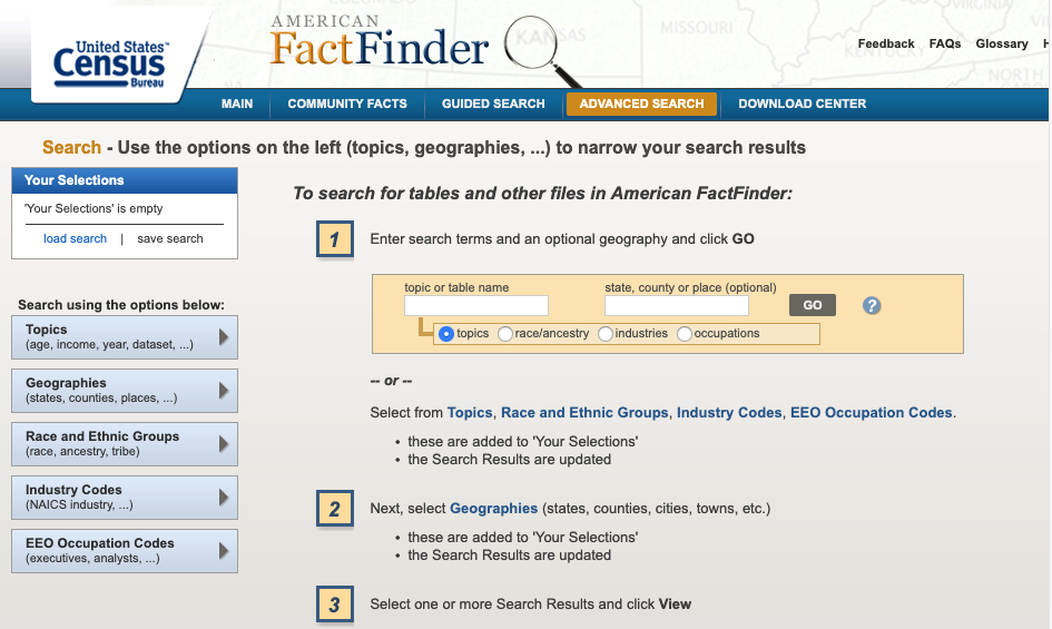
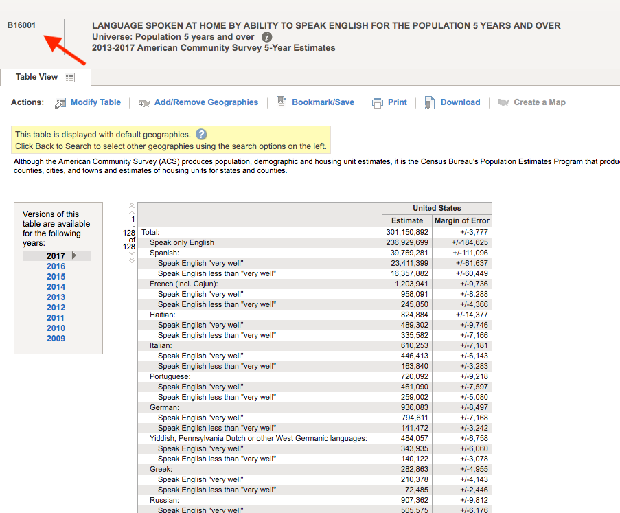
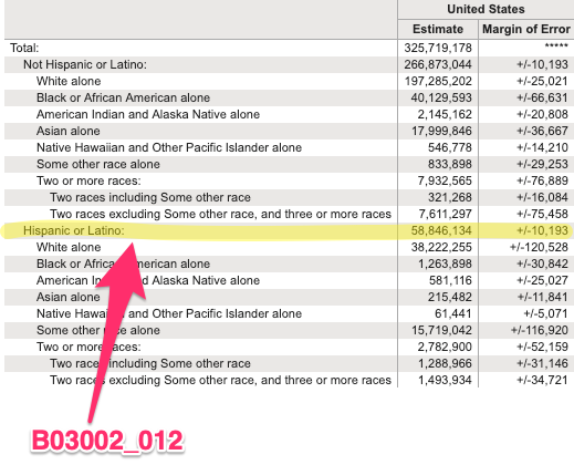
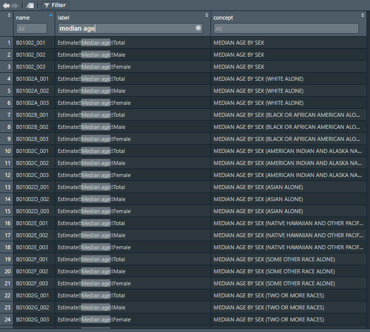
Using tidycensus to work with Census data

# Using tidycensus to work with Census data
### Sono Shah
### (updated: 2019-07-23)

---

## Slides:

## https://sonoshah.github.io/tidycensuspresentation/slides

## Code:

## https://sonoshah.github.io/tidycensuspresentation/examples.r

---

# What is Tidycensus?

## It's an R package that allows for interfacing with the US Census Bureau's **decennial census** and **ACS** APIs.

---

# FactFinder & DataFerrett Pain

![](ff-screenshot.png)
]

## Do you regularly have to use FF to pull down the same table (i.e. B02001) for **multiple levels of geography** or for **multiple years**?

---

# Benefits of Tidycensus

- ## You can reduce the amount of **"point-and-click"**

- ## reproducibility, and scale

- ## It is **tidyverse-friendly** (easily integrate the **`%>%`**)

- ## Supports downloading spatial data (aka shapefiles so you can easily make maps)

---

# What kinds of data can I get?

- [American FactFinder Tables](https://factfinder.census.gov/faces/nav/jsf/pages/index.xhtml)
  
--

- American Community Survey
  - 1-yr, 3-yr, and 5-yr 
  - Years **2010 - 2017** 
  
--

- decennial census
  - 1990, 2000, and 2010

- population estimates
  - population, components, housing, and characteristics

---

# What you can do with tidycensus?

---

# Go from Data to table or visualization quickly

```r
get_acs(geography = "state",
         variables = "B03002_012",
        year = 2017,
        survey = "acs1",
        summary_var = "B03002_001") %>% 
  head(10)
```

```
## Getting data from the 2017 1-year ACS
```

```
## The one-year ACS provides data for geographies with populations of 65,000 and greater.
```

```
## # A tibble: 10 x 7
##    GEOID NAME              variable  estimate   moe summary_est summary_moe
##    <chr> <chr>             <chr>        <dbl> <dbl>       <dbl>       <dbl>
##  1 01    Alabama           B03002_0…   201970  2353     4874747          NA
##  2 02    Alaska            B03002_0…    51712   110      739795          NA
##  3 04    Arizona           B03002_0…  2202173    NA     7016270          NA
##  4 05    Arkansas          B03002_0…   223764  1357     3004279          NA
##  5 06    California        B03002_0… 15477306    NA    39536653          NA
##  6 08    Colorado          B03002_0…  1206724    NA     5607154          NA
##  7 09    Connecticut       B03002_0…   578833    NA     3588184          NA
##  8 10    Delaware          B03002_0…    89540    NA      961939          NA
##  9 11    District of Colu… B03002_0…    76526    NA      693972          NA
## 10 12    Florida           B03002_0…  5370860   461    20984400          NA
```

---

# To a Table

<div id="htmlwidget-2e9b4be710a2d406f681" style="width:100%;height:auto;" class="datatables html-widget"></div>
<script type="application/json" data-for="htmlwidget-2e9b4be710a2d406f681">{"x":{"filter":"none","data":[["California","Texas","Florida","New York","Illinois"],[15477306,11158751,5370860,3811654,2206927],[0.391467279741662,0.394238130090251,0.255945368940737,0.192028685604033,0.172388926343907]],"container":"<table class=\"display\">\n  <thead>\n    <tr>\n      <th>NAME<\/th>\n      <th>Hispanic Population<\/th>\n      <th>Share Hispanic<\/th>\n    <\/tr>\n  <\/thead>\n<\/table>","options":{"dom":"t","columnDefs":[{"className":"dt-right","targets":[1,2]}],"order":[],"autoWidth":false,"orderClasses":false,"rowCallback":"function(row, data) {\nDTWidget.formatCurrency(this, row, data, 1, '', 0, 3, ',', '.', true);\nDTWidget.formatPercentage(this, row, data, 2, 0, 3, ',', '.');\n}"}},"evals":["options.rowCallback"],"jsHooks":[]}</script>

---

```r
* get_acs(geography = "county",
        variables = "B03002_012",
        year = 2017,
        survey = "acs1",
        summary_var = "B03002_001") %>%
* top_n(10,wt = estimate)
```

]

]

---

# What I'll show you

- ## How to install tidycensus

- ## How to pull data

- ## How to pull data with shape files (for mapping!)

---

# How to install tidycensus

### 1. Visit **https://api.census.gov/data/key_signup.html** and sign up for an API key (it's free!)

### 2. Start R/Rstudio and install the package using **`install.packages("tidycensus")`**

### 4. Load the package using **`library(tidycensus)`**

### 5. Install your census key and use option `install = TRUE`.

```r
census_api_key("PASTE-YOUR-KEY-HERE",install = TRUE)
```

## You are ready to start pulling data!

]

---

# Main Functions

- ### `get_acs()`: American Community Survey

- ### `get_decennial()`: Decennial Census

- ### `get_estimates()`: Population Estimates
  
- ### `load_variables()`: Load variables to search in R
  
---

# Using `get_acs`

- ### **geography**: i.e. `state`, `US`, `county` `school district`, etc.

- ### **year**: endyear of sample i.e. `2017`

- ### **survey**: i.e. `acs1`, `acs5`

- ### **table** or **variables**: i.e. `B03002` or `B03002_012`

---

# Why use **variables** instead of a table ID?

---

# Why use **variables** instead of a table ID?

![](ff-b03002-2.png)
]

---

- ## In other instances you might have a single row, but you need to pull tables with different suffixes (i.e. Median Household Income)

- B19013D = Median HH Income (Asian Alone HH)
  - B19013H = Median HH Income (NH-White Alone HH)
  - B19013I = Median HH Income (Hispanic, any race HH)
  
---

# Why use **variables** instead of a table ID?

## Instead of pulling each table separately, you can pull them all together like this:

```r
get_acs(geography = "county",
*       variables = c("B19013D_001","B19013H_001","B19013I_001"),
        year = 2017,
        survey = "acs1",summary_var = "B19013_001") %>% 
  top_n(n = 10,wt= summary_est)
```

---
 
# Supported Geographies

- ### US

- ### Region

- ### State, County, tract, block group, place, congressional district, zip code, school district

- ### pretty much anything you might want.

.footnote[Full list of options available [here](https://walkerke.github.io/tidycensus/articles/basic-usage.html)]

---

# Looking up variables

- What if you are not a crazy person and you don't know the table number from memory?

- NO PROBLEM! We can look it up using the `load_variables()` function

```r
load_variables(year = 2017,dataset = "acs5")
```

]

---

classes: inverse

```r
get_acs(geography = "county",
        state="CA",
        county = "037",
*       variables =c("B19013_001",
*                    "B19013B_001",
*                    "B19013D_001",
*                    "B19013H_001",
*                    "B19013I_001"),
        year = 2017,
        survey = "acs1")
```

]

<img src="slides_files/figure-html/unnamed-chunk-9-1.svg" width="504" />
]

---

# Using `summary_est` to calculate proportions

- We want data on the top 5 congressional districts with the largest population share of:
  - Hispanics
  - Asians
  - Blacks
  
- To make calculations easier, we can set `summary_var` to = the total population of the congressional district.
  
---

# Using `summary_est` to calculate proportions

- Here's what the code looks like

```r
groupstopull <- c("B03002_003","B03002_004",
                  "B03002_006","B03002_012")
get_acs(geography = "congressional district",
*       variables = groupstopull,
        year = 2017,
        survey = "acs1",
*       summary_var = "B03002_001")
```

]

```
## Getting data from the 2017 1-year ACS
```

```
## The one-year ACS provides data for geographies with populations of 65,000 and greater.
```

```
## # A tibble: 8 x 4
## # Groups:   group [4]
##   NAME                    group    estimate group_share
##   <chr>                   <chr>       <dbl>       <dbl>
## 1 District 5, Kentucky    NH-White   669225       0.961
## 2 District 6, Ohio        NH-White   656627       0.943
## 3 District 40, California Hispanic   650436       0.881
## 4 District 34, Texas      Hispanic   618721       0.850
## 5 District 2, Mississippi Black      470765       0.671
## 6 District 9, Tennessee   Black      462385       0.663
## 7 District 17, California Asian      425657       0.552
## 8 District 1, Hawaii      Asian      355195       0.497
```
]

---

classes: inverse, middle

# Pull data over time

---

- Using `get_estimates` we can pull data from the Census population estimates API

```r
* get_estimates(geography = "combined statistical area",
*              product = "population",
              year = 2018,
*              time_series = T)
```

]

```
## # A tibble: 10 x 5
##    NAME                        DATE GEOID variable   value
##    <chr>                      <dbl> <chr> <chr>      <dbl>
##  1 Albany-Schenectady, NY CSA     1 104   POP      1168485
##  2 Albany-Schenectady, NY CSA     2 104   POP      1168490
##  3 Albany-Schenectady, NY CSA     3 104   POP      1168881
##  4 Albany-Schenectady, NY CSA     4 104   POP      1169036
##  5 Albany-Schenectady, NY CSA     5 104   POP      1170182
##  6 Albany-Schenectady, NY CSA     6 104   POP      1171186
##  7 Albany-Schenectady, NY CSA     7 104   POP      1171074
##  8 Albany-Schenectady, NY CSA     8 104   POP      1170599
##  9 Albany-Schenectady, NY CSA     9 104   POP      1169677
## 10 Albany-Schenectady, NY CSA    10 104   POP      1171448
```
]

---

<img src="slides_files/figure-html/unnamed-chunk-14-1.png" width="504" height="80%" />
]

---

# Mapping

- Tidycensus also has support for pulling census boundary data.

- This can be great for some quick prototyping

- You can download the spatial data by setting `geometry = TRUE` when pulling data.

---

```r
ca_tract_geo <- get_acs(geography = "tract",
               state="CA",
               variables = "B19013_001",
*              geometry = T)
head(ca_tract_geo)
```

- Notice the extra column

```
## Simple feature collection with 6 features and 5 fields
## geometry type:  MULTIPOLYGON
## dimension:      XY
## bbox:           xmin: -122.2694 ymin: 37.83454 xmax: -122.2124 ymax: 37.88544
## epsg (SRID):    4269
## proj4string:    +proj=longlat +datum=NAD83 +no_defs
##         GEOID                                          NAME   variable
## 1 06001400100 Census Tract 4001, Alameda County, California B19013_001
## 2 06001400200 Census Tract 4002, Alameda County, California B19013_001
## 3 06001400300 Census Tract 4003, Alameda County, California B19013_001
## 4 06001400400 Census Tract 4004, Alameda County, California B19013_001
## 5 06001400500 Census Tract 4005, Alameda County, California B19013_001
## 6 06001400600 Census Tract 4006, Alameda County, California B19013_001
##   estimate   moe                       geometry
## 1   208393 46352 MULTIPOLYGON (((-122.2469 3...
## 2   147500 34827 MULTIPOLYGON (((-122.2574 3...
## 3    88173 11036 MULTIPOLYGON (((-122.2642 3...
## 4   102821 13517 MULTIPOLYGON (((-122.2618 3...
## 5    92375 18444 MULTIPOLYGON (((-122.2694 3...
## 6    86458 30610 MULTIPOLYGON (((-122.2681 3...
```

---

```r
ca_tract_geo %>% 
  ggplot(aes(fill = estimate)) + 
  geom_sf(color = NA) + 
  coord_sf(crs = 26911) + 
  scale_fill_viridis_c(option = "plasma",
                       labels=scales::dollar) +
  theme_minimal()+
  labs(title = "Tract-Level HH Median Income",
       fill = "HH Median Income")
```

]

]

---

```r
ca_tract_geo %>% 
  filter(str_detect(NAME,"Riverside County")) %>% 
  ggplot(aes(fill = estimate)) + 
  geom_sf(color = NA) + 
  coord_sf(crs = 26911) + 
  scale_fill_viridis_c(option = "plasma",
                       labels=scales::dollar) +
  theme_minimal()+
  labs(title = "Tract-Level HH Median Income",
       fill = "HH Median Income")
```

]

]

---

# Uses

- Create r scripts for "top 10 counties/states/zipcodes/whatever"

- Build a Shiny App that connects to Census APIs for internal use

- Quickly pull down contextual data for merging into surveys

---

# Other random things

- [Margin of Error estimates + calculator](https://walkerke.github.io/tidycensus/articles/margins-of-error.html)

- Tidycensus comes with a built-in dataset called `fips_codes` which has county name, fips code, state name, state fips code, state abbrev.

- Tiycensus gives you the option of formmating the data as "long" versus "wide", using option `output = "wide"`.

---

classes: inverse

# Helpful Links for Tidycensus

- [TidyCensus Documentation](https://walkerke.github.io/tidycensus/index.html)

- [Pulling Multi-Year Data](https://mattherman.info/blog/tidycensus-mult-year/)

- [Kyle Walker Data](https://walkerke.github.io/)

---

classes: inverse

# Helpful links for Tidycensus

- [Pull all tracts for US](https://walkerke.github.io/2017/05/tidycensus-every-tract/)

- [Mapping with Leaflet](https://juliasilge.com/blog/using-tidycensus)

- [Mapping with TMAP](http://zevross.com/blog/2018/10/02/creating-beautiful-demographic-maps-in-r-with-the-tidycensus-and-tmap-packages/)

- [Working with Census data in R](https://rconsortium.github.io/censusguide/)

---

classes: inverse

# Other Tools

- Do you use IPUMS data? There's an R package for that https://cran.r-project.org/web/packages/ipumsr/vignettes/ipums.html

- Other R packages for Census

- `censusapi` gives access to 300+ Census APIs https://github.com/hrecht/censusapi
  
  - `lehdr` gives access to the Longitudinal Employer-Household Dynamics data (LODES) https://github.com/jamgreen/lehdr

- [Tabula](https://tabula.technology/) - Extract Tables from PDFs

- [Tabulizer](https://cran.r-project.org/web/packages/tabulizer/vignettes/tabulizer.html) - Same thing but as an R package for programatic use!

---

# The end

## Slides:

## https://sonoshah.github.io/tidycensuspresentation/slides

## Code:

## https://sonoshah.github.io/tidycensuspresentation/examples.r